Intrinsic vs. Extrinsic Geometry and The Metric Tensor Illustrated

We illustrate the metric tensor as a mathematical book-keeping device which accounts for the variable change necessary in converting “ground-distance” to “hiking-distance” in a topographical map. Calculations are done in topographical maps to re-enforce the intuitive explanation given of intrinsic and extrinsic geometry.

Last Updated: Wednesday, January 03, 2024 - 12:30:17.

Imagine Collecting the Following Materials:

1. a flat piece of thick, gray construction paper,
2. a thin piece of pink, semi-transparent tracing paper,
3. and a yellow spotlight…on the lens of which…
4. …you have drawn a star in black Sharpie pen.

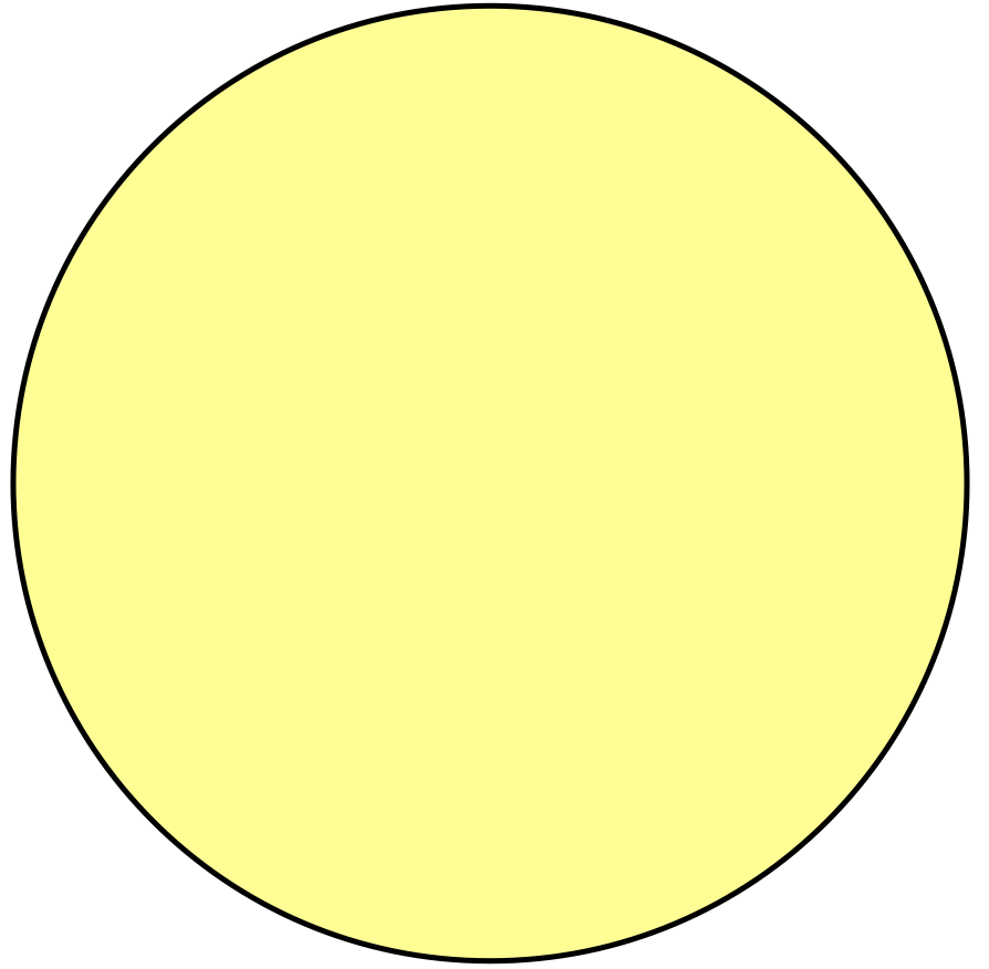
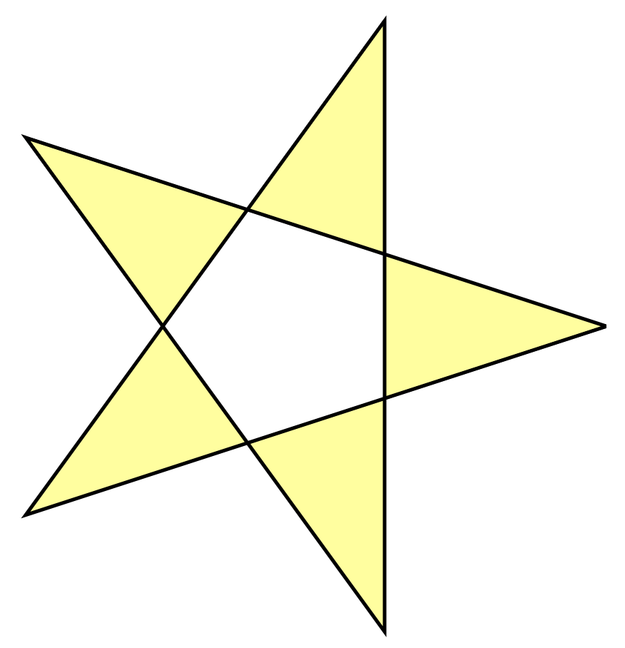
Figure 1: Some Materials You Have Collected to Develop an Idea about Intrinsic vs. Extrinsic Geometry

Imagine Using These Collected Materials:

• Clear a space to work in your messy office or bedroom.
  
• Lay the gray construction paper on the floor or a desk.
  
• To get some practice with a pair of scissors you have found, you cut the pink tracing paper into a circle.
  
• Now, in one hand, hold this pink circle above the gray paper but between the spotlight which you hold in your other hand.
  
• With this setup, as seen in Figure 2, you notice that the star on the flashlight casts a star-shaped shadow onto not only the semi-transparent pink tracing paper but also through onto the gray construction paper below.

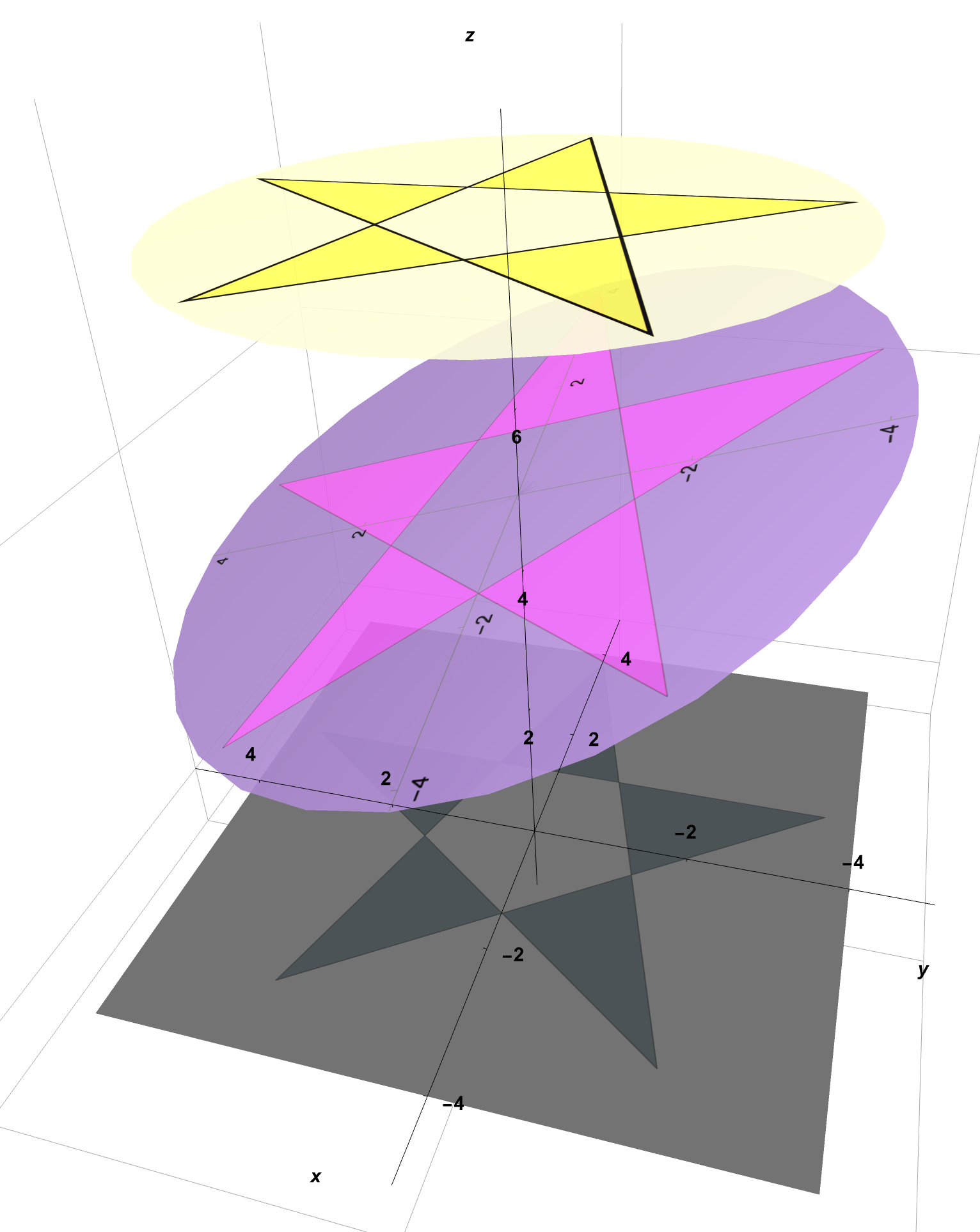
Figure 2: Here is What You Created With Your Collected Materials. The Star on the Yellow Spotlight Casts a Shadow on the Pink Transparent Paper and Then Onto the Gray Paper Below

While searching the internet for interesting shapes…

You happen upon a shape called a Helicoid (seen in Figure 3) which, on a first pass, looks like just a twisted version of a piece of paper. You find, however, that you are unable to construct this twisted shape from a single piece of pink tracing paper without creating wrinkles or tears. However, with a significant amount of time, patience, scissors, and glue, you are able to construct a reasonable approximation of this helicoid from many small pieces of pink paper. With this newly constructed helicoidal shape, you set up your shadow casting apparatus again. This time, as you rotate the resulting helicoid around its central axis in space, you notice that the spotlight illuminates only the portions of the surface that are accessible to the light.

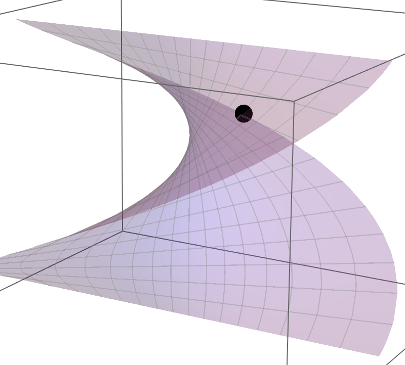
Figure 3: You Want Your Paper to Take the Shape of this “Helicoid”.

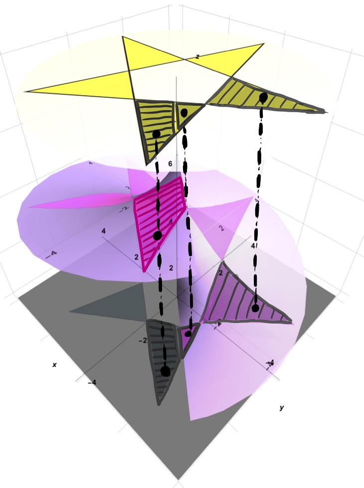
Figure 4: Shadow As a Projection. Only the parts of the surface that come into contact with the light rays (vertical dotted lines) coming from the spotlight are illuminated.

Extrinsic Geometry in the Shadow-Casting Context:

This situation, in essence, reflects the Extrinsic Geometry of the surface, namely, features of the surface can be exposed by some external methods of space. That is, the shadow cast onto the surface exists only because the spotlight was first present in space to create the light which then interacted with the surface itself in space to create this shadow. Any questions we wish to ask about the surface (for example, those distance and angle questions in Figure 5) can be asked instead of the shadow cast onto this surface from the spotlight in space. These questions about the shadow on the surface can then be answered with the understanding that the tools and techniques of space are at our disposal (e.g. rulers, tape measures, and string to find lengths and protractors to measure angles).

Figure 5: Questions We Wish to Ask About the Surface Like the Distance Between Two Points A and B Along a Path 1 -> 2 -> 3 -> 4 or Like the Measure of One of the Angles of a Projected Triangle on a Surface Can Be Answered Using the Shadow Cast Onto This Surface From the Spotlight in Space. These questions can be answered with rulers, string, and protractors which are some tools of space.

An Experiment with Photosensitive Paper:

Given your success constructing a helicoid out of tracing paper, you decide to repeat the construction with yellow, photosensitive paper. Repositioning the star above this new construction, you leave the photosensitive paper to develop an image while you go and get coffee. Upon returning some time later, you find the following image imprinted onto the helicoid as seen in Figure 6 which prompts some natural questions. Some time later, sufficiently tired from constructing and thinking about how to make distance and angle computations without spatial tools you fall asleep wondering about the meaning of Intrinsic Geometry…

(… and this is what you dream…)

a star \once remembered \easily forgotten

a supernova \ captured \ nuclear afterimage

yourself \ miniscule \ trapped in crepuscular corona

perception\ sun-blinded \ claustrophobic

fate\ restricted \ a struggle to know more

Upon waking you realize that a way to make sense of your dream is to imagine yourself being trapped as a photographic image onto a helical surface made of photosensitive paper, and that in this transference you retain no knowledge of your prior existence in three-dimensional space. While this seems rather claustrophobic, you at least have retained the ability to move within the surface using your two remaining degrees of freedom (known to a 3D spatial observer as the width and vertical directions of the helicoid, but known to you the photographic inhabitant as simply \(v\) (moving across or left/right in the surface) and \(u\) (moving forward/backward on the surface), respectively.

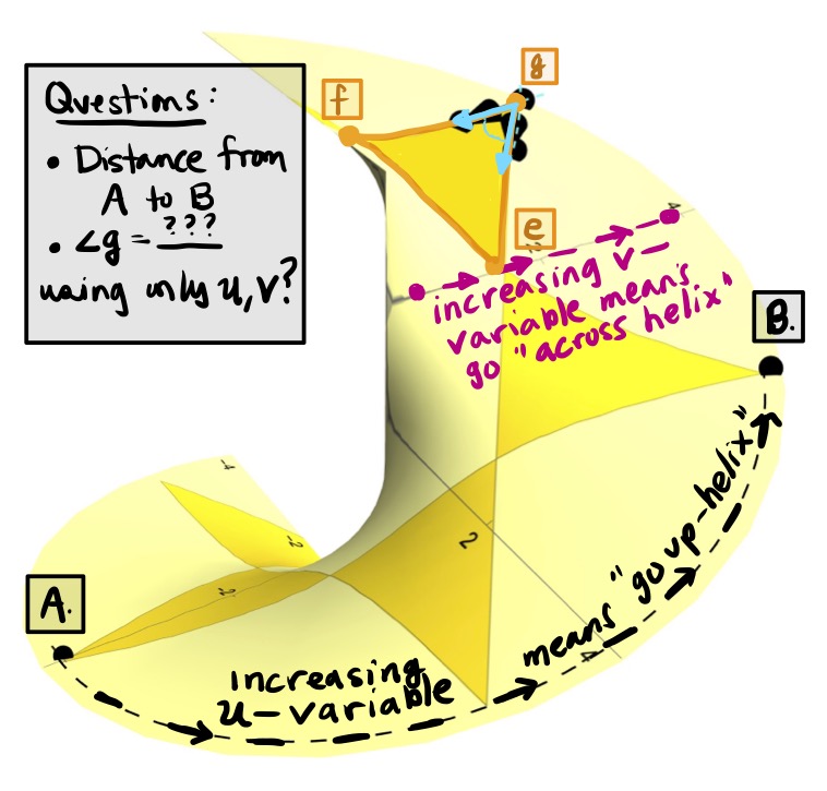
Figure 6: Instead of Transparent Pink Tracing Paper, Procure Some Yellow Photosensitive Paper. Leave this photosensitive paper exposed to the spotlight, and you will find the star photographically imprinted onto the helicoidal, photosensitive paper. The star now rotates with the helicoid as the star is now inseparable from the surface itself.

Intrinsic Geometry in Photographic Terms:

Intrinsic Geometry then are those features of the surface that can be discovered while being “photographically embedded” into the surface. Intrinsic geometry requires that knowledge of surface be discovered using intrinsic tools that are developed with no reference to or knowledge of the surfaces prior extrinsic existence in space. Intrinsic tools should be constructed from knowledge of the variables \(u\) and \(v\) and special functions thereof (for example, the metric tensor \(g_{\alpha \beta}\)).

It turns out that, as hinted at in Figure 7, despite a transference to the photographic paper, special knowledge of an intrinsic object called the metric tensor \(g_{\alpha\beta}\) can be obtained, which allows one to compute lengths and angles in this new, restricted (intrinsic) surface environment defined by the vectors \(\partial_{1}=\partial_{u}\) and \(\partial_{2}=\partial_{v}\).

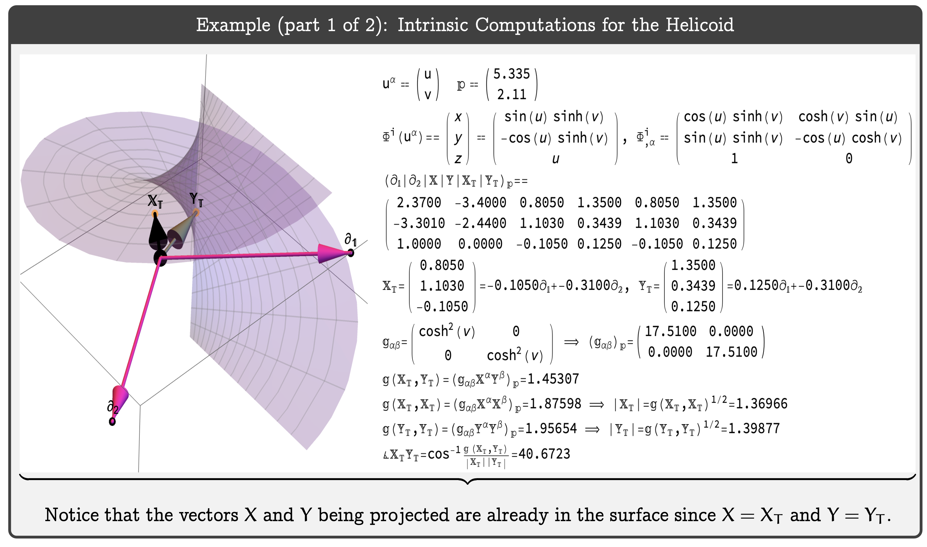
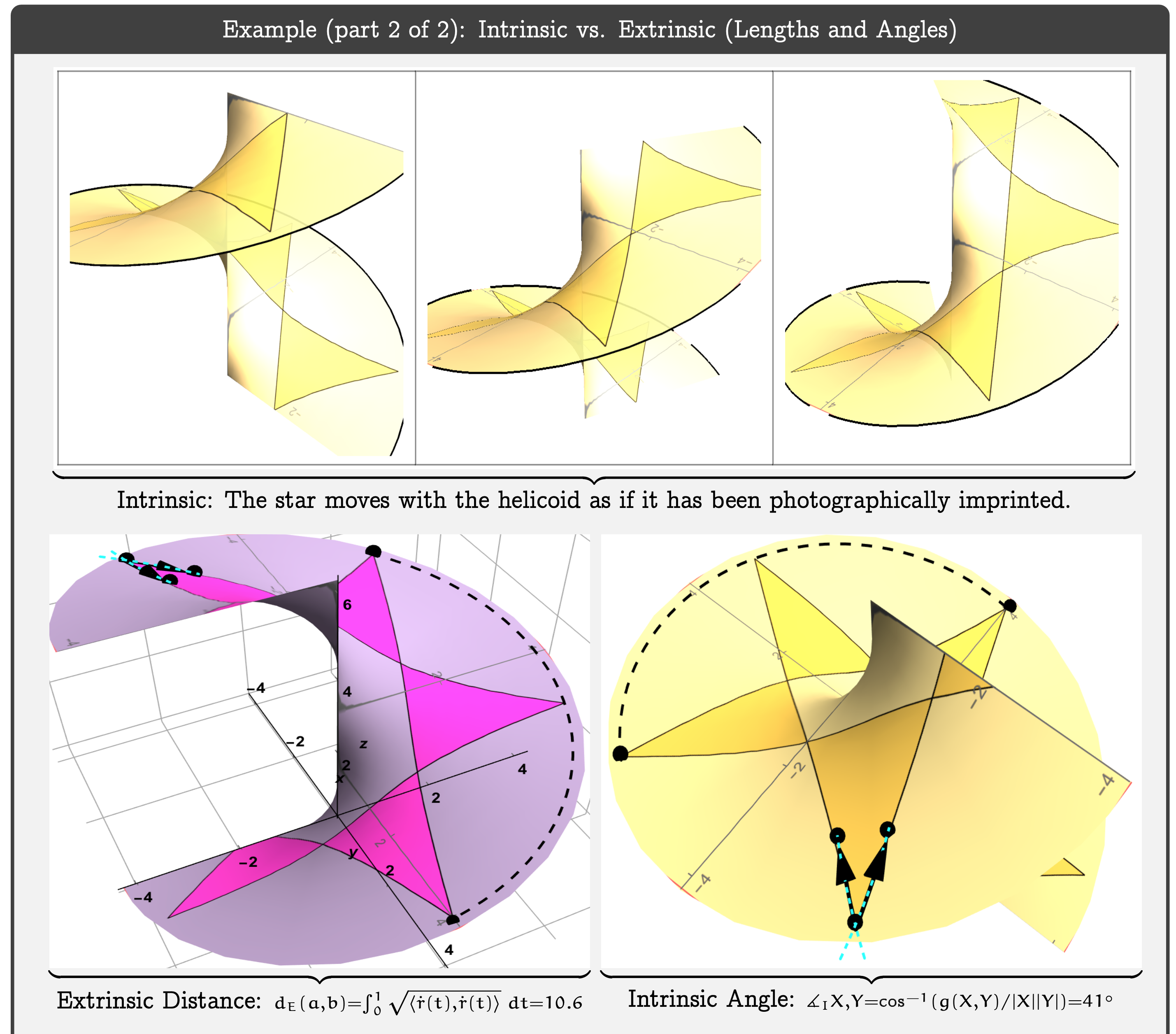
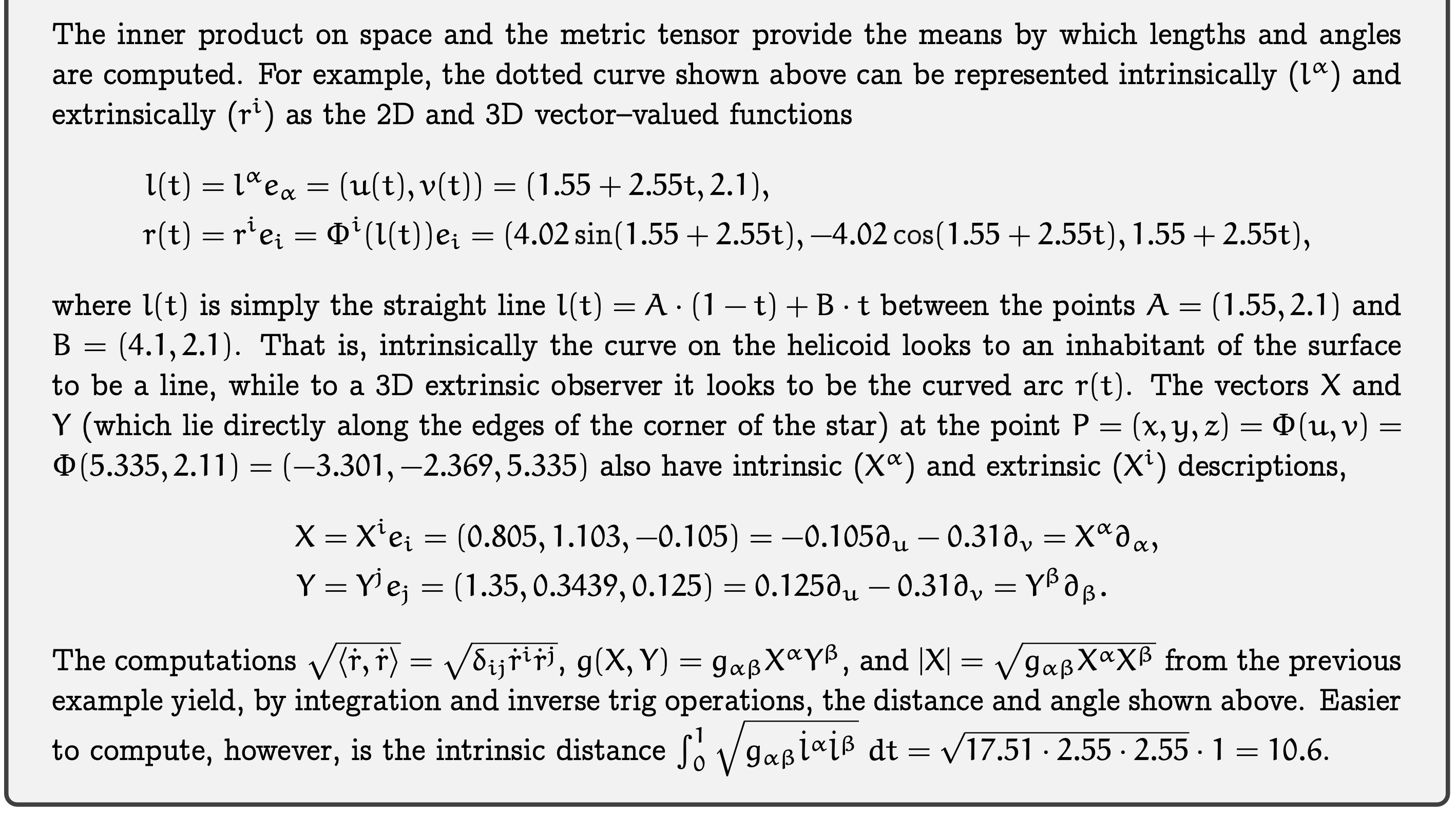
Figure 7: Screenshots of Intrinsic Computations with the Metric Tensor. Details to follow in the additional resources (Apple Book, YouTube Video, etc.) to this post.

A Step, Skip, and a Jump Towards Metrics…

Using the metric tensor of the Helicoid (as seen in Figure 7) to compute lengths and angles intrinsically in the surface is not yet that satisfying as we have not yet developed the intuition behind the concept of Metrics. To develop this intuition and to step, skip, and jump towards the concepts of intrinsic geometry and the metric tensor, consider the illustration of a race shown in Figure 8.

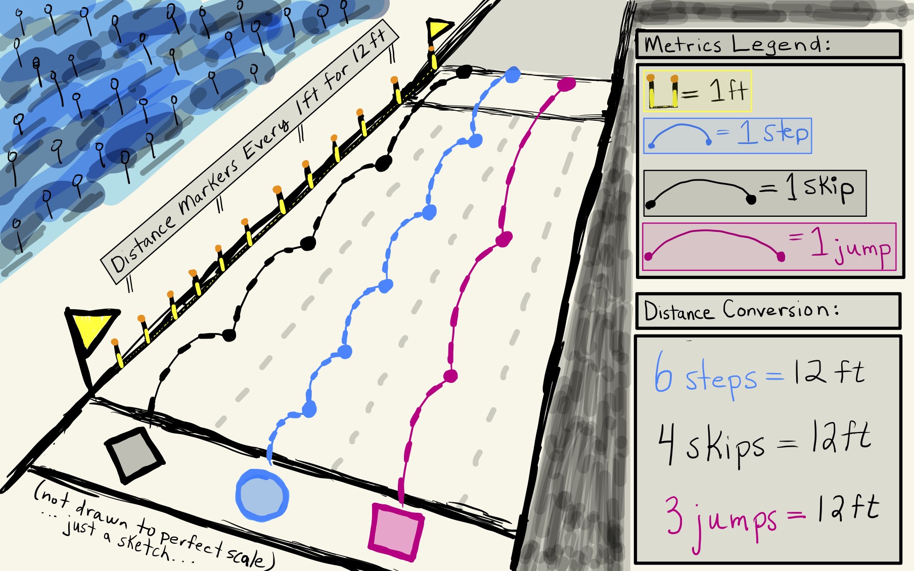
Figure 8: Imagine a Race with Three Contestants: The first (blue) contestant is a Stepper, which means they can only take Steps towards the finish line. The second (black) contestant is a Skipper, and thus wants to try to complete the race with Skips. The third (pink) contestant is a Jumper who is sure that this athletic ability will allow them to win the race. The race begins! According to one outside (extrinsic) observer in the crowd, they see a straight track that is 12ft in length which the blue contestant completes by taking 6steps at 2ft per step. To a second outside observer the black contestant complete the race in 4skips at 3ft per skip, while a third observer watches in amazement as the jumper complete the course in just 3 jumps at 4ft per jump. The contests tie!. They all completed the 12ft course at the same time albeit with different racing methods (or Metrics).

Metrics Definition…

According to one definition of Metrics obtained from the internet:

Metrics (/metriks/)

(…a method of measuring something) Each race contestant (the intrinsic observers) had a different method for measuring the length of the race based on their chosen racing mode or metric (6steps or 4skips or 3jumps). In contrast, the race fans (the extrinsic observers) had their own metric in the form of the race markers on the outside of the track (12ft).

(…the results obtained from this) This form of the definition is interesting as it can help us see the race, not really as a race, but as a means of dividing up the track into smaller parts. Imagine every time one of the contestants foot touches the ground (after a Step, a Skip, or a Jump) that a line across the track is made visible for the fans. By the end of the race, we might then see something like shown in Figure 10 or that seen from a top view in Figure 11.

Figure 9: Metrics Definition: a method of measuring something, or the results obtained from this.

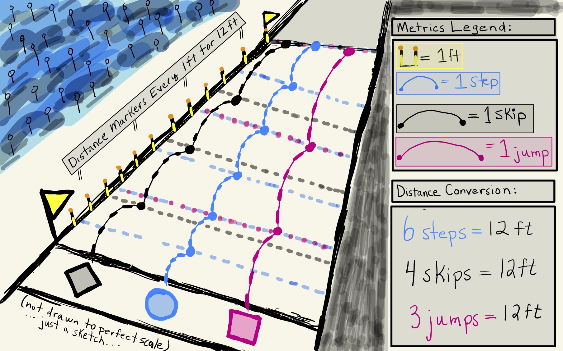
Figure 10: Imagine the Race as a Means of Dividing the Track into Smaller Parts.

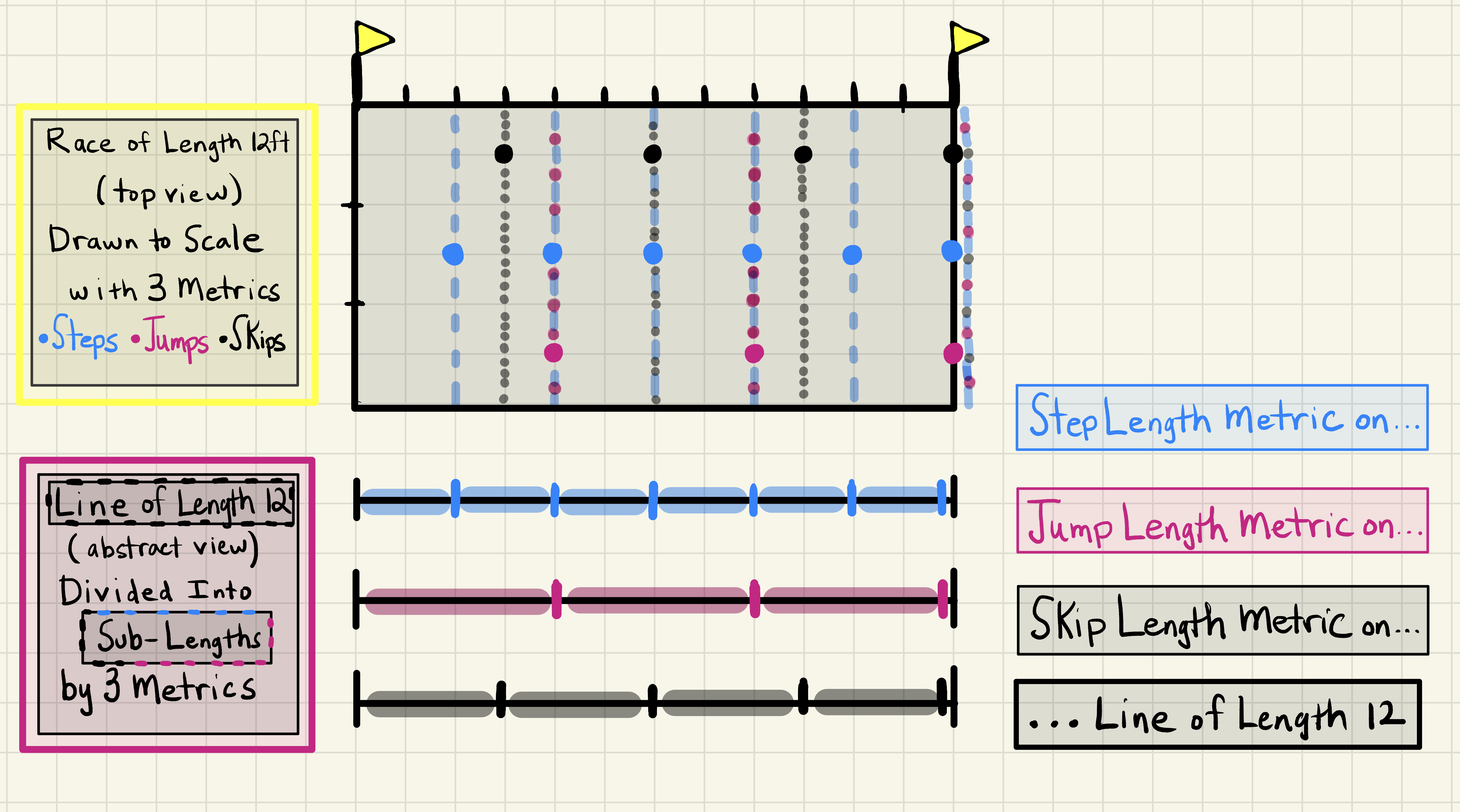
Figure 11: Top View of Track Divided into Smaller Parts Using Three Fixed Metrics

A Variable Metric and Race Summary:

Imagine now that one race fan (extrinsic) decides that they want to be a fourth contestant in what they know to be the 12ft race. As a now contestant (intrinsic) they decide to mix and match the race modes (fixed metrics) from the previous contestants into their own varying metric as shown in Figure 12. To summarize the four race completion strategies we have:

• (Stepper, Step Metric) 6steps
• (Skipper, Skip Metric) 4skips
• (Jumper, Jump Metric) 3jumps
• (Former Observer, New Contestant, Variable Metric) 2skips, 1step, and 1jump

Because the New Contestant was a Former Observer who had the extrinsic knowledge that 1step=2ft, 1skip=3ft, and 1jump=4f, it follows that the contestants as a group are able to compare their intrinsic metrics (steps, skips, jumps, variable) to the extrinsic metric (ft) to see that they have all actually traveled the same distance of 12ft:

• (Stepper) \[\begin{equation*} 6steps \cdot \frac{2ft}{1step}=6\cdot 2ft=12ft \end{equation*}\]
• (Skipper) \[\begin{equation*} 4skips \cdot \frac{3ft}{1skip}=4\cdot 3ft=12ft \end{equation*}\]
• (Jumper)

\[\begin{equation*}3jumps \cdot \frac{4ft}{1jump}=3\cdot 4ft=12ft\end{equation*}\]

• (Variable)

\[\begin{align*} & \left(2skips \cdot \frac{3ft}{1skip}\right) \\ &+\left(1step \cdot \frac{2ft}{1step}\right) \\ &+\left(1jump\cdot \frac{4ft}{1jump}\right)\\ &=6ft+2ft+4ft\\ &=12ft\end{align*}\]

The concept of a variable metric extends from the length of a racetrack to distances traveled on a curved surface. The surface can be viewed as a mountainous park as seen in Figure 13

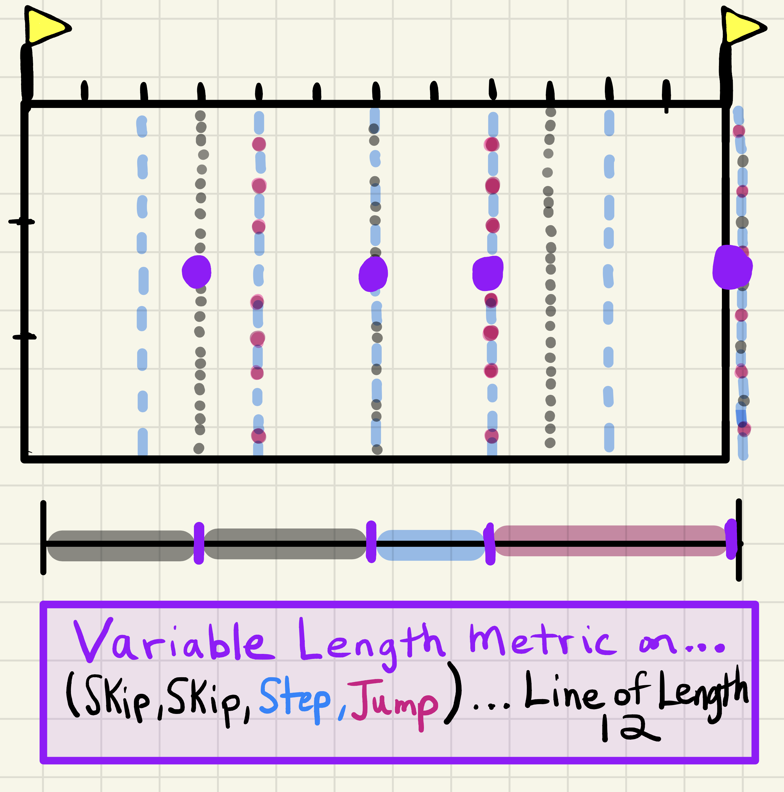
Figure 12: Top View of Track Divided into Smaller Parts Using A Variable Metric

Imagine a Surface as a Mountainous Park:

In this next several sections we introduce and motivate the idea of the metric tensor \(g_{\alpha \beta}\) of a surface using the, perhaps, more familiar concept of the topographical map the surface.

Figure 13: Imagine a Surface as a Mountainous Park.

Imagine A Mountainous Park as a Topographical Map:

To make a topographical map of a surface, consider drawing many planes of constant elevation. As seen in Figure 14, the intersection of these planes with the surface create the constant elevation or contour curves of the surface. Drawing many contour curves together on a single plot is the topographical map of the surface as seen for example in Figure 15

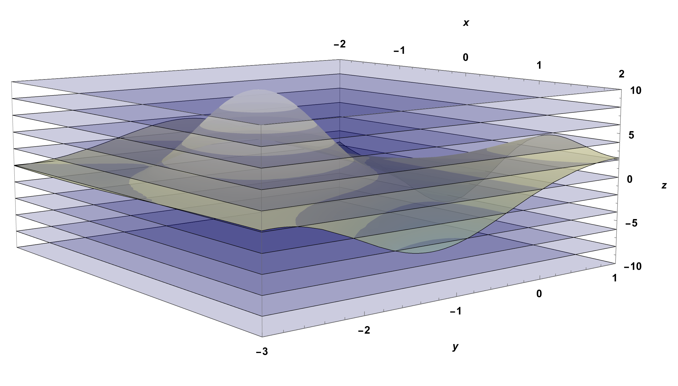
Figure 14: Creating a Topographical Map of a Surface. Step 1: Draw many planes of varying, constant elevations. Here the elevations are set to be every 2 units on the z-axis. Step 2: Where these planes intersect the surface become the curves of constant elevation (contour curves). Crossing from a contour curve to one other (next) contour curve means you have changed elevation by 2 units of vertical distance.

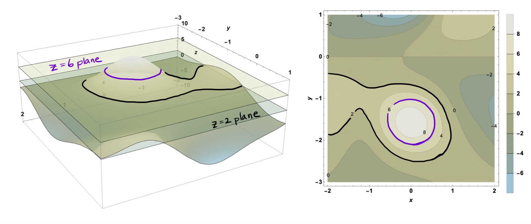
Figure 15: Step3: Drawing many contour curves together on a single plot is a topographical map of the surface. The spacing of the contour curves in this topographical map correspond to a vertical change of 2 units of distance.

The Park Could Have Many Sections and Many Trails:

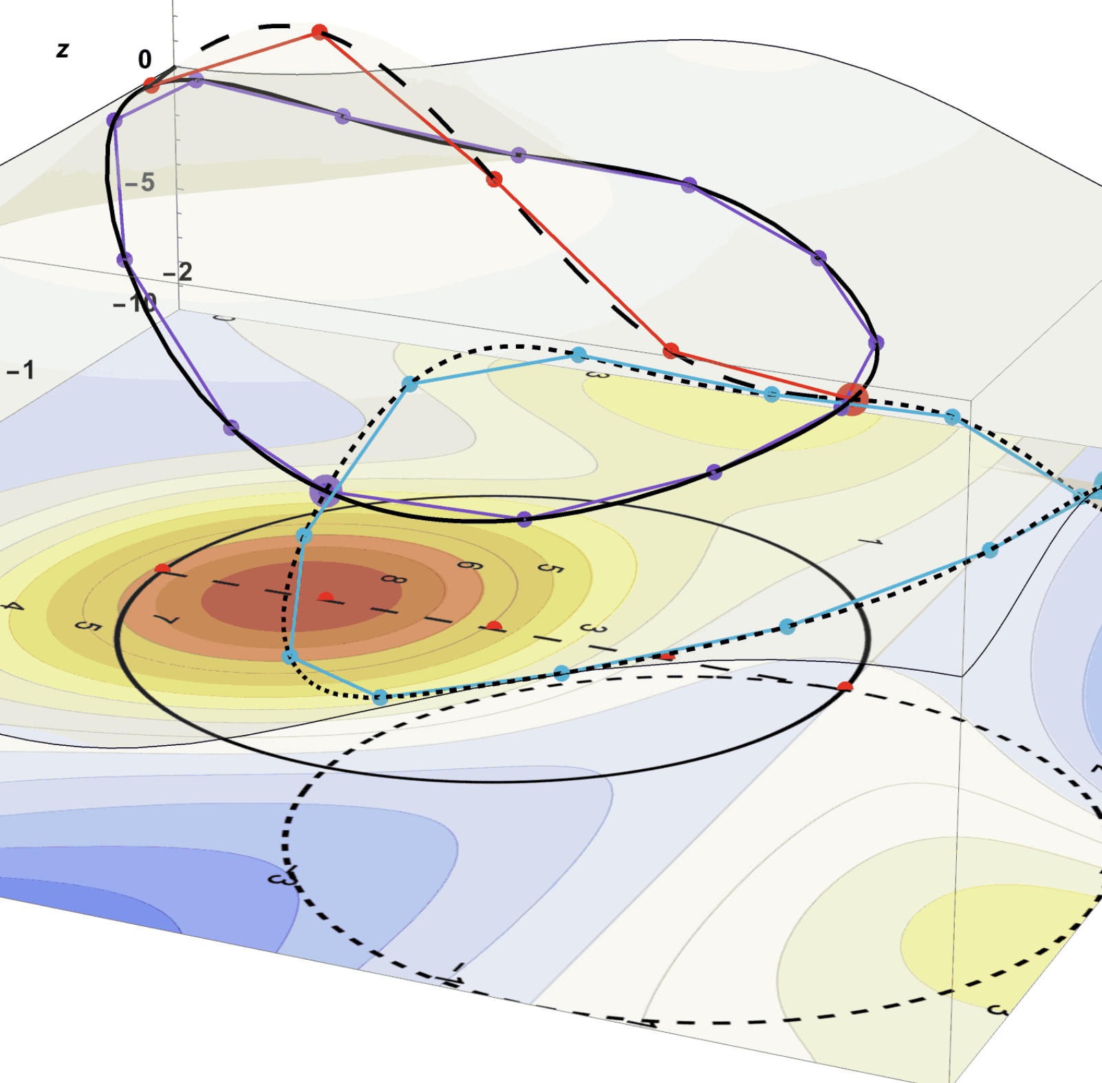
The section on the park you have chosen to go to has three possible trails. In an effort to be prepared for whichever trail you might use, you have brought a variety topographical maps of a varying degrees of detail of the different regions as seen in Figure 16 which are shown in the context of the park itself in Figure 17. Imagine the whole mountainous park to be the size of your topographical maps and imagine the trails shown by their trail marker colors (Red for the Peak Trail, Purple for the Mountain Loop Trail, and Blue for the Valley Loop Trail).

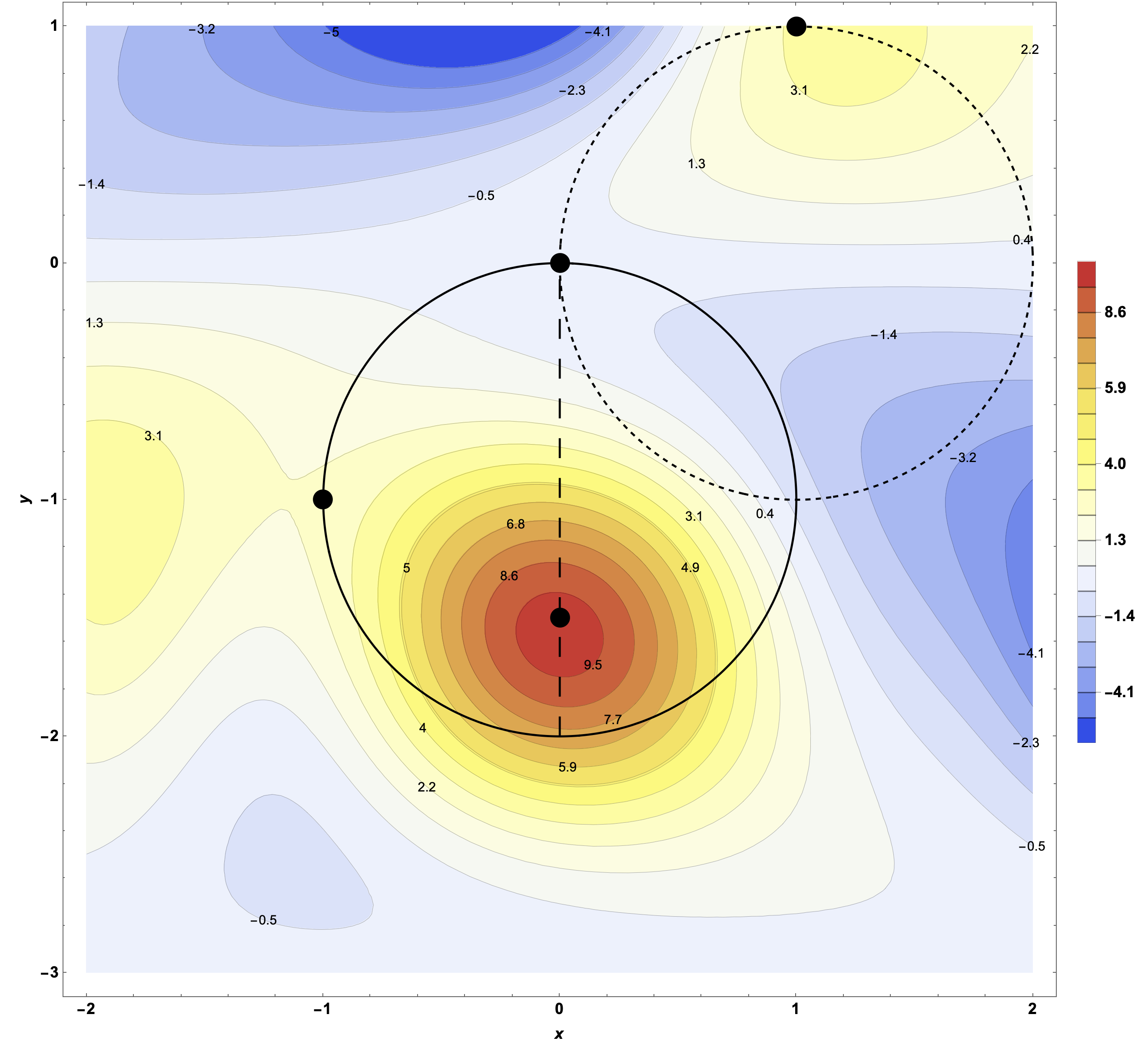
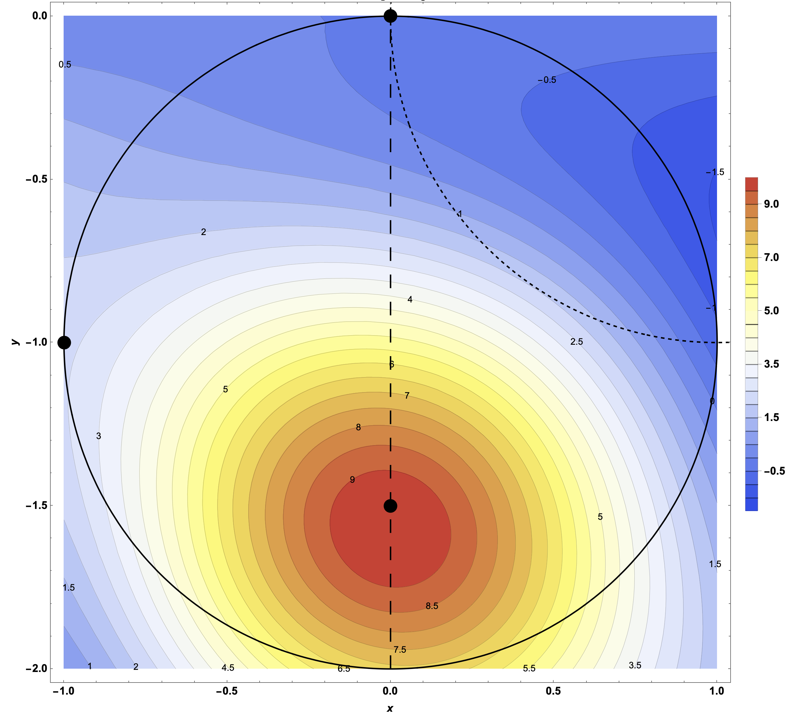
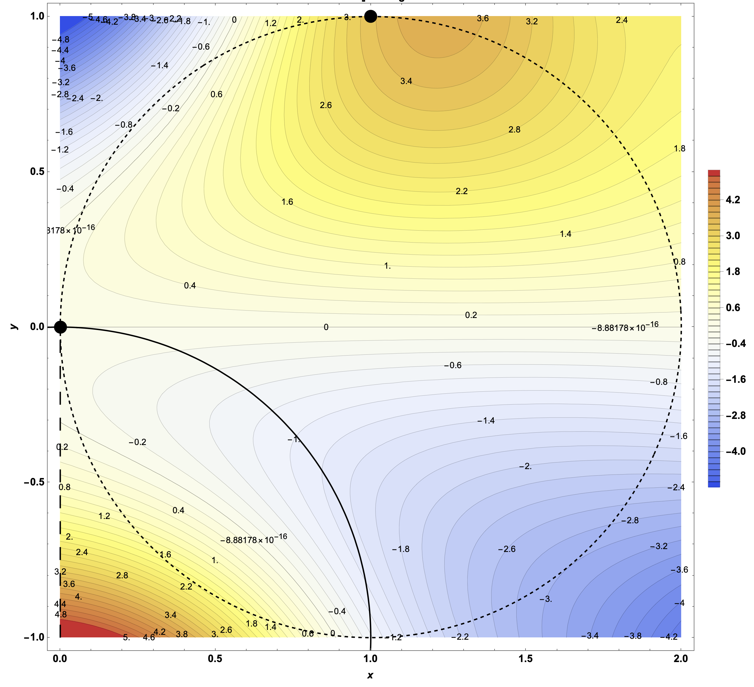
Figure 16: You Have a Variety of Topographical Maps of the Area. The topographical maps of the park show flattened versions of the surrounding hilly terrain. On these maps, the colors and numbers correspond to the elevations above or below the parks office (which is considered to be elevation 0).

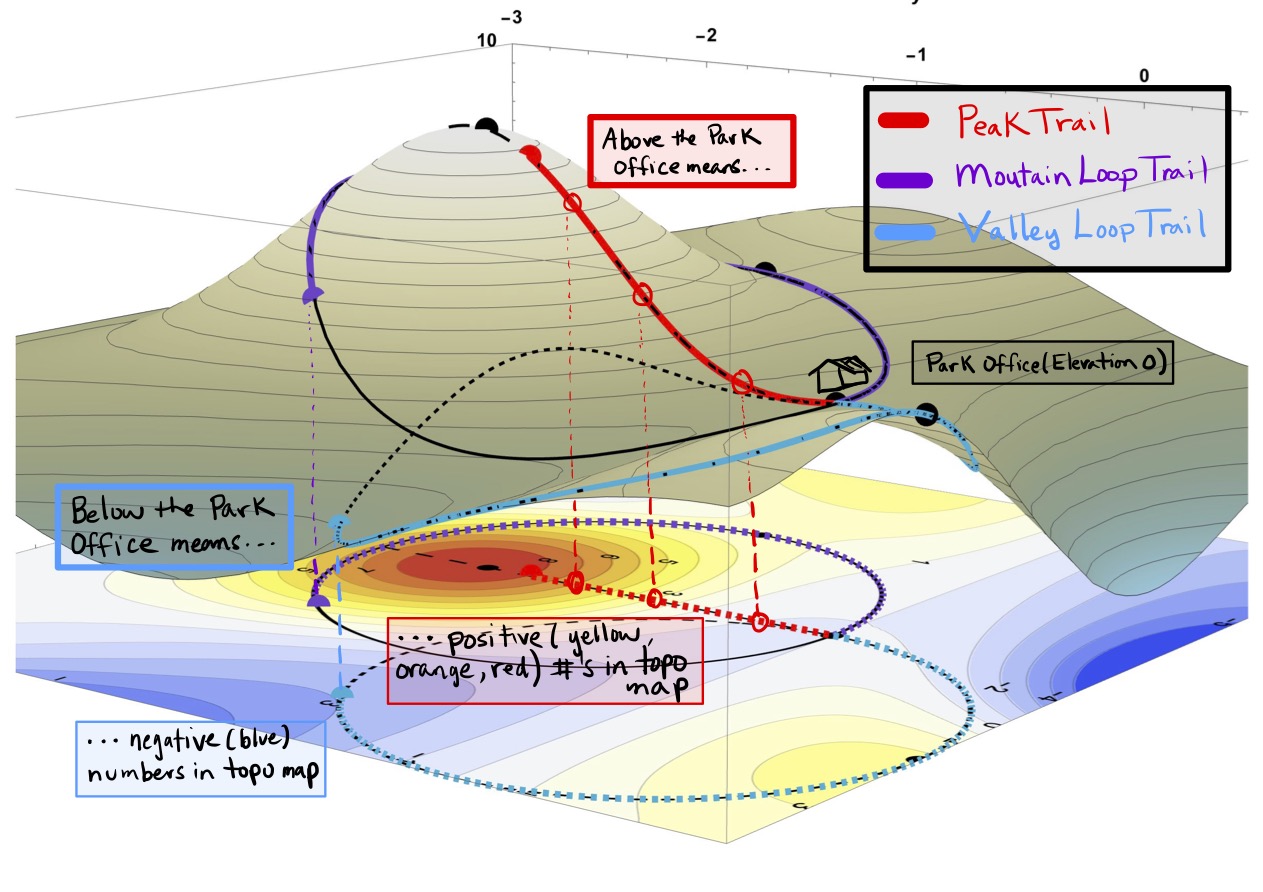
Figure 17: The Relationship of the Topographical Map to the Surface. Imagine the whole mountainous park to be the size of your map and imagine the trails shown by their trail marker colors (red for the Peak Trail, purple for the Mountain Loop Trail, and blue for the Valley Loop Trail). Hiking the red Peak Trail means following the red dotted path on the topographical map which will take you to high (red) elevations around 8 above the park office. Hiking the purple Mountain Loop means following the purple dotted path on the map with some elevations in the yellow range around 5 above the park office. The blue Valley Loop follows the blue dotted path on the map which leads to some elevations in the blue range around 3 below the park office.

The Walking Distances Between Points on the Mountain Depends on the Trail:

The computation of distances between points on the mountainous surface along different paths can be accomplished using the data contained in the corresponding topographical maps. Understanding the spacing of the constant elevation (or contour) curves of the surface is a key to the metric tensor \(g_{\alpha\beta}\) of the surface, and therefore the computation of distances between points along paths.

Figure 18: Distance Computations Between Points on the Surface Can Be Accomplished Using the Elevation Data in the Corresponding Topographical Map.

How to Incorrectly Compute Walking Distance to Tip-Top of Peak Trail (and What You Could Try Instead):

Walking the Peak Trail to the TipTop seen in Figure 19 presents a great opportunity to show how to incorrectly compute walking distance using the Pythagorean Theorem as illustrated in Figure 20. Recall the Pythagorean Theorem (for computing the length of the hypoteneuse, \(c\)) of a right triangle whose leg lengths are \(a\) and \(b\)

\[\begin{align*} c=\sqrt{a^{2}+b^{2}}. \end{align*}\]

Figure 19: Walking the Peak Trail to the Tip-Top Shows a Total Walking Distance of 10.41 units.

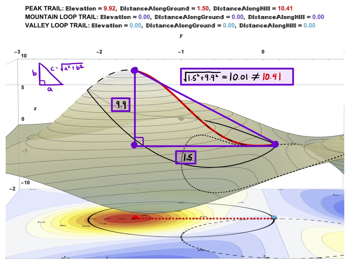
Figure 20: In Trying to Understand Where a Total Walking Distance of 10.41 Comes From, It is Incorrect to Just Use the Pythagorean Theorem. Using this method in this case undercomputes the walking distance.

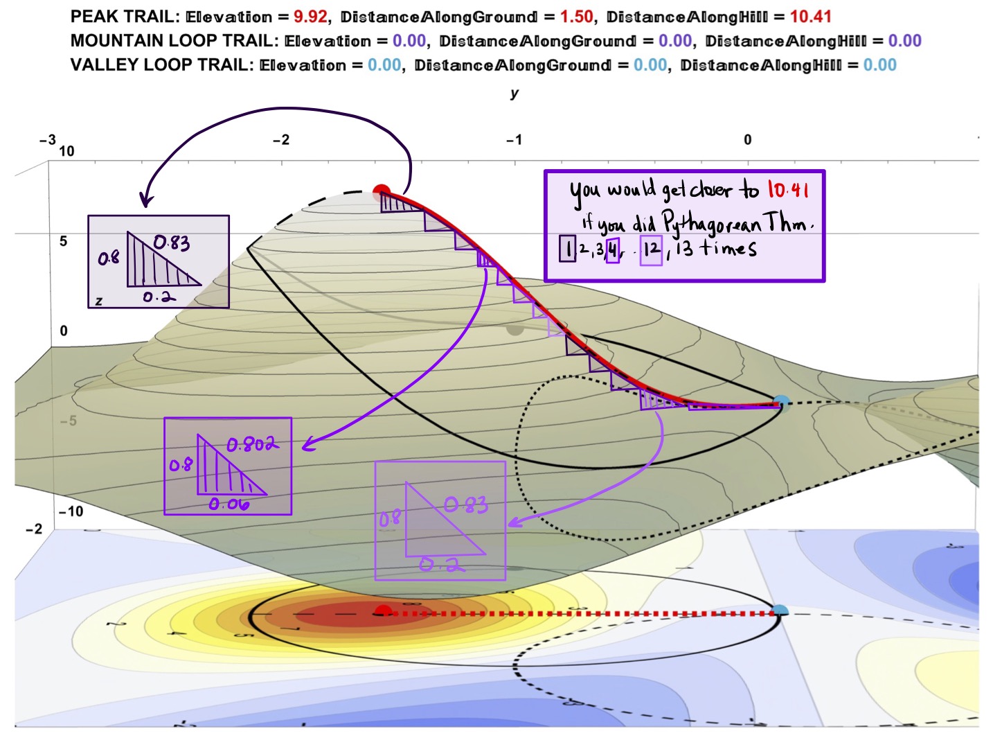
Figure 21: In Trying to Understand Where a Total Walking Distance of 10.41 Comes From, It Would Be More Correct to Use the Pythagorean Theorem Multiple Times.

Trail Distances Can Be Approximated Using Repeated Pythagorean Theorem:

A common problem solving strategy in mathematics is to reduce a complicated problem (like the exact distance measurement problem) into smaller, less complicated problems (like the problem of finding the length of a single line segment). The trade off in solving these less complicated problems is that there are usually many, many of these smaller problems to need to be “re-assembled” to find final answer to the complicated problem (like needing to add the lengths of many line segments together to get a total curve length).

Figure 22: Walking All the Trails and Exact Distances. For the Time Being, Assume These Exact Distance Measurements Come From the Pedometer Readings of Your Smart Watch.

Figure 23: Approximate Distances by Dividing the Trails Into Many Straight-Line Segments. The Lengths of Straight Lines are Straight-Forward (pun intended).

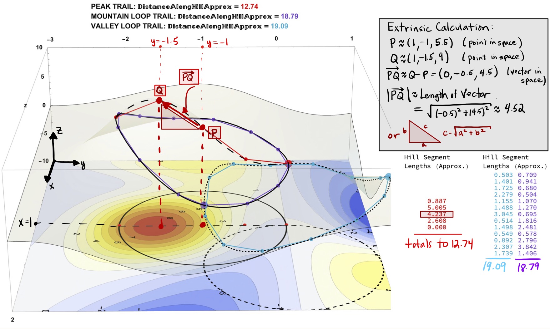
Figure 24: Extrinsic Computations for the Lengths of Vectors in Space are Performed with Pythagorean’s Theorem.

The Smaller the Line Segments Used the Better the Trail Distance Approximation:

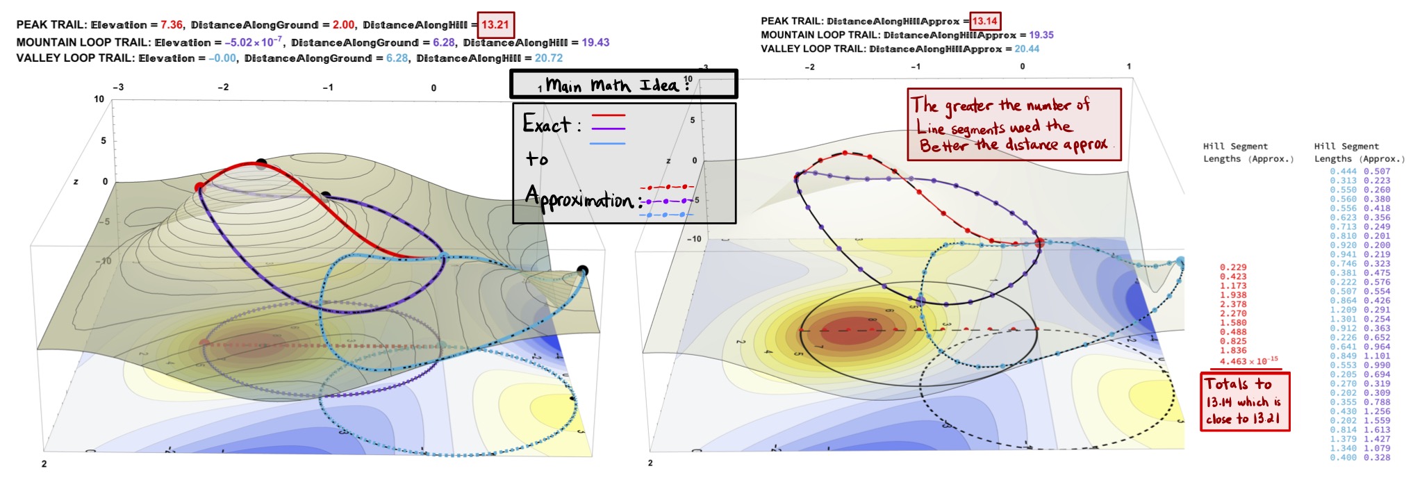
Figure 25: (A Common Problem Solving Strategy) The Exact Distance Measurements Along the Trails on the Mountainous Surface (left) Can Be Approximated by Adding the Lengths of Many Straight-Line Segments (right). The More Segments Used the Better the Approximation.

Find Walking Distances on Trails Using Contour Lines:

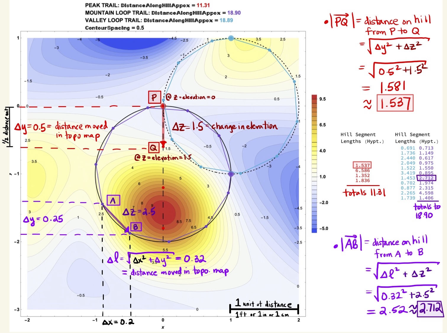
Figure 26: Distances Along Line Segments of the Trails are Found with Repeated Application of the Pythagorean Theorem (to compute the Length of the Hypotenuse).

Towards a Variable Distance Metric for Tip-Top Peak Trail…Similar to the Step, Skip, Jump Race

This section illustrates the connection between the variable metric idea introduced in section A Variable Metric and Race Summary: with a variety of topographical map calculations. By dividing the trail into sequentially smaller segments on which we perform extrinsic calculations for elevation gains and hiking distances, we create a reasonable approximation of a variable metric on the Peak Trail which motivates a more detailed treatment of in section The Metric Tensor:.

Figure 27: Consider the Segment Length Data for the Tip-Top Trail: This Length Data Partly Required Extrinsic Knowledge of the Elevation Data.

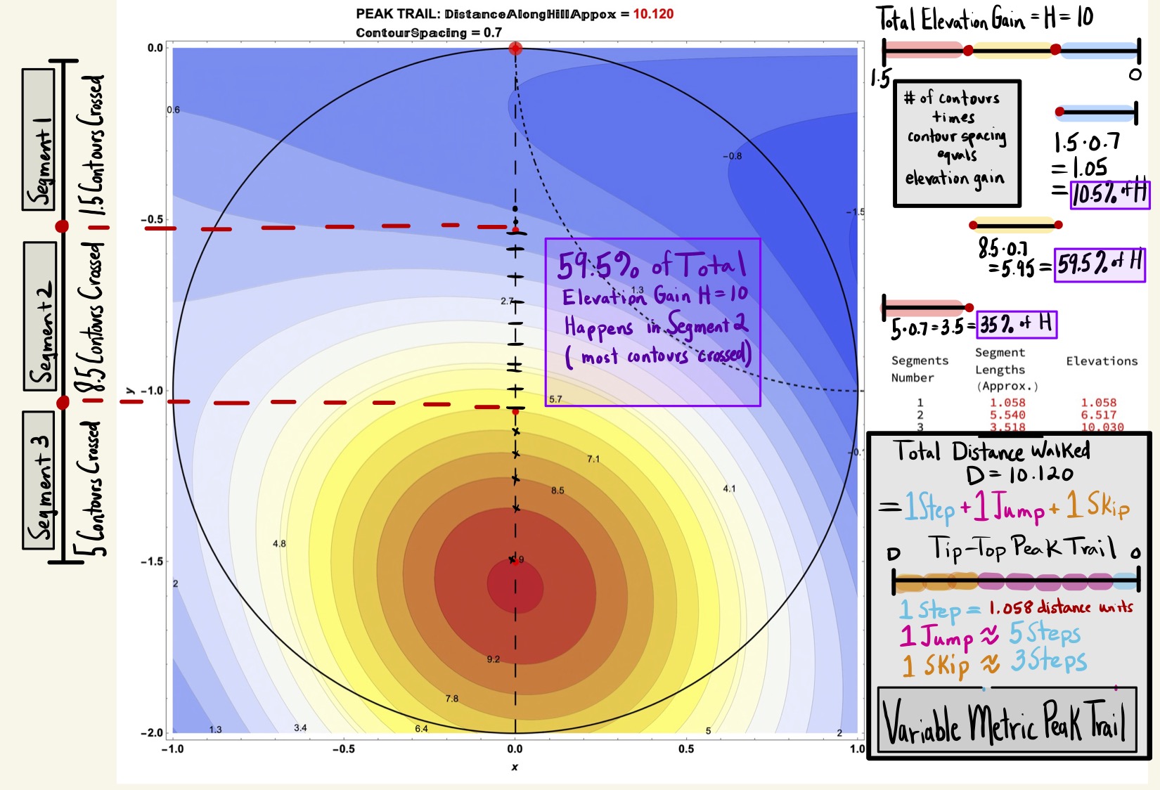
Figure 28: Consider the Segment Length Data for the Tip-Top Trail (0.7 Contour Spacing, 3 Segments with Spacing 0.5).

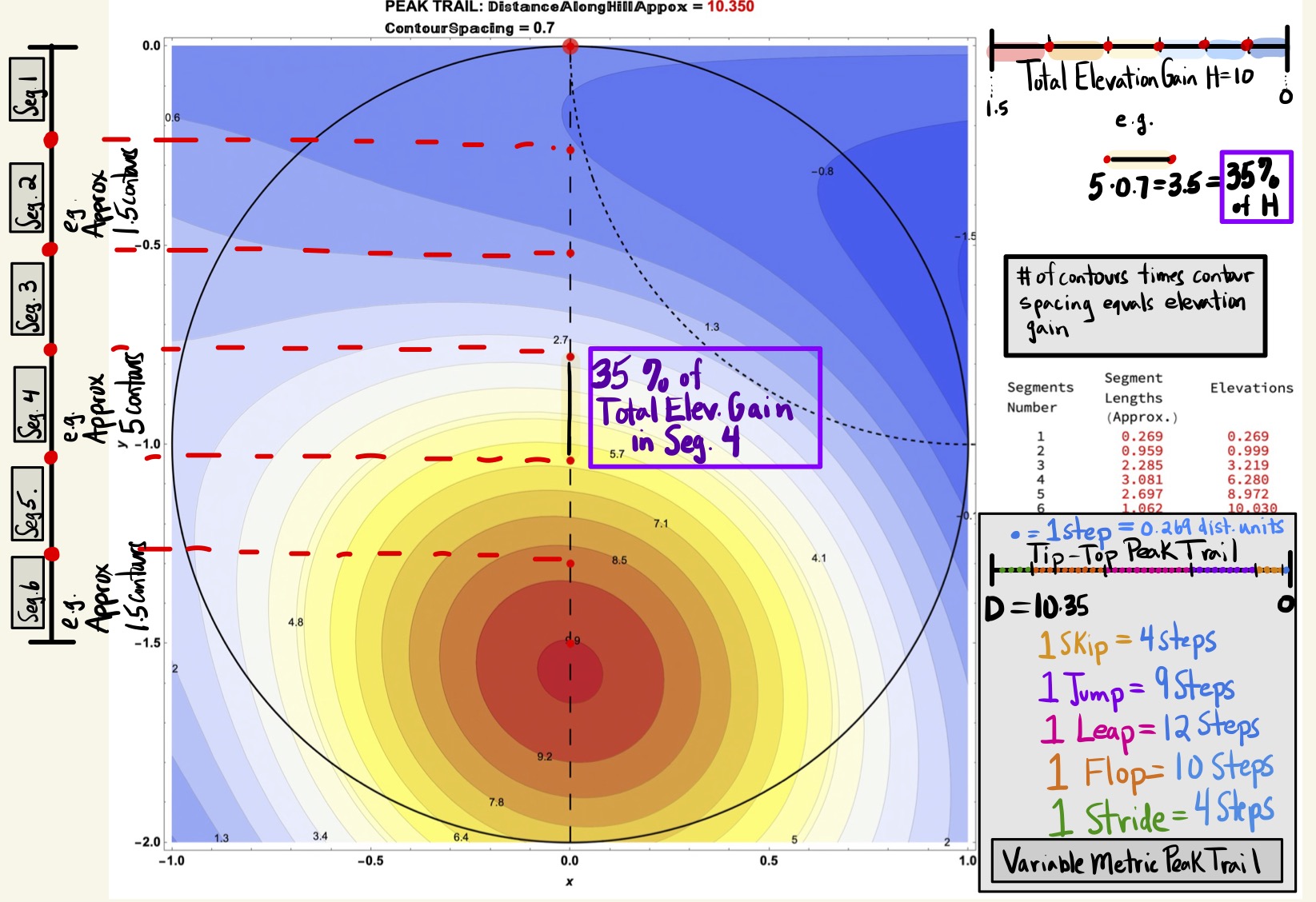
Figure 29: Consider the Segment Length Data for the Tip-Top Trail (0.7 Contour Spacing, 6 Segments with Spacing 0.25).

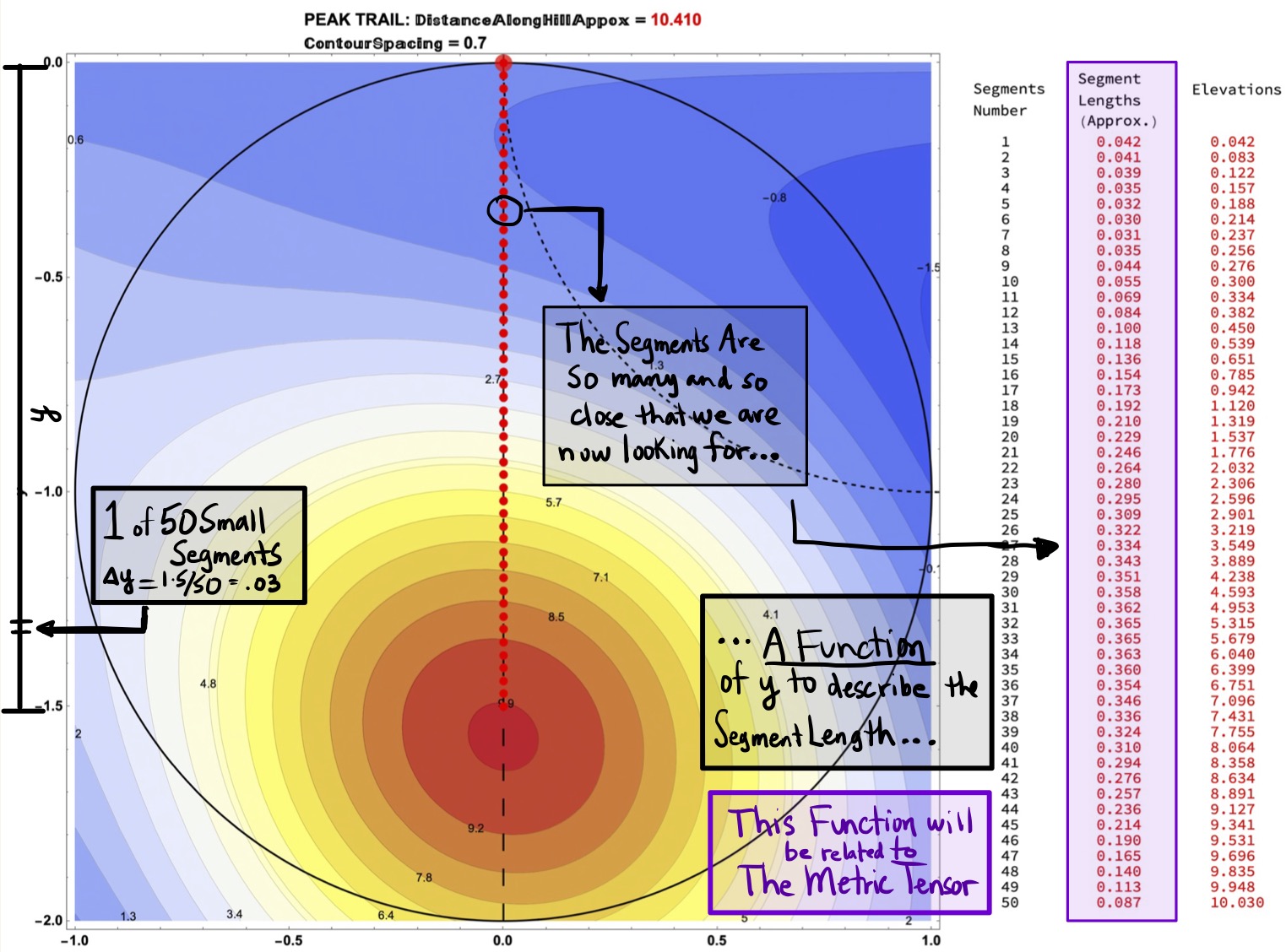
Figure 30: Consider the Segment Length Data for the Tip-Top Trail (0.7 Contour Spacing, 50 Segments with Spacing 0.03).

The Metric Tensor:

In this section we transition from extrinsic to intrinsic calculations of distance by using the metric tensor as a scale factor which converts “along-the-ground-distance” to “along-the-trail-distance”. We see that as the number of trail segments increases, then intrinsic and extrinsic computations of distance converge to each other.

The metric tensor \(g_{\alpha\beta}\) of a surface written as \(z=f(x,y)\) is the matrix

\[\begin{align*} g_{\alpha\beta}=\begin{pmatrix} g_{11} & g_{12} \\ g_{21} & g_{22} \end{pmatrix}=\begin{pmatrix} 1+f_{x}^{2} & f_{x}f_{y} \\ f_{x}f_{y} & 1+f_{y}^2 \end{pmatrix} \end{align*}\]

where \(f_{x}\) and \(f_{y}\) are the partial derivatives of the surface equation \(z=f(x,y)\) with respect to \(x\) and \(y\). In the case of our mountainous park, the \(z\)-values (or elevations) can be obtained by \((x,y)\) location in the park by the equation

\[\begin{align*} f(x,y)&=-10 \cos ^3(x) \sin ^3(y)+\cos (x) \sin (y) \cos ^2(y)\\ &+2 \sin (x) \sin (y) (\cos (x) \sin (y)+1)^2\\ &+3 \sin (x) \sin (y) \cos (y) \end{align*}\]

from which the the metric tensor \(g_{\alpha\beta}(x,y)\) follows at any point in the park \((x,y)\). This matrix is quite complicated due to the complicated nature of the terrain. However, the metric tensor along the Peak Trail given by the points \((x,y)=(0,y)\) can be reduced to simply to a function of \(y\) \[\begin{align*} g_{\alpha\beta}(y)=\begin{pmatrix} g_{11}(y) & g_{12}(y) \\ g_{12}(y) & g_{22}(y) \end{pmatrix}, \end{align*}\]

where

\[\begin{align*} g_{11}(y)&=\left(2 \sin (y) (\sin (y)+1)^2+3 \sin (y) \cos (y)\right)^2+1\\ g_{12}(y)&=\left(\cos ^3(y)-32 \sin ^2(y) \cos (y)\right)\\ &\cdot \left(2 \sin (y) (\sin (y)+1)^2+3 \sin (y) \cos (y)\right)\\ g_{22}(y)&= \left(\cos ^3(y)-32 \sin ^2(y) \cos (y)\right)^2+1. \end{align*}\]

The Figures 31 and 32 show that intrinsic computations of (hill) segment length can be obtained from ground distance \(\Delta y\) and (the square root of) the metric tensor \(\sqrt{g_{22}(y)}\) by a scale factor formula:

\[\begin{align*} \mbox{Hill Segment Length}=\Delta y \cdot \sqrt{g_{22}(y)}. \end{align*}\]

The Peak Trail, because of its constant southerly heading (with no east-west deviation), is an ideal example to use since only one component of the metric tensor is needed \(g_{22}\) for scaling. Intrinsically computing the walking distance on this specific trail nicely illustrates the metric tensors role as a mathematical book-keeping device accounting for the variable change necessary in converting “ground-distance \(\Delta y\)” to “hill-distance, \(\Delta y \cdot \sqrt{g_{22}(y)}\)”. The metric tensor stores intrinsically all the information necessary to ensure that extrinsic computations of distance match the intrinsic distance.

Figure 33 shows that as \(\Delta y\) decreases to \(0\) (and therefore the number of segments increases to \(\infty\)) the intrinsic and extrinsic segment lengths begin to converge. So too then do the trail distances converge (aka the totals of the segments lengths).

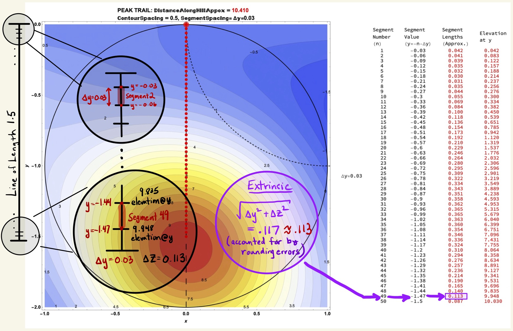
Figure 31: Definitions of \(y\), \(\Delta y\), and \(\Delta z\) Needed to Extrinsically Compute Segment Lengths.

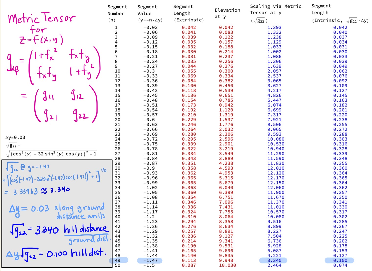
Figure 32: Definition of Metric Tensor \(g_{\alpha \beta}\) and Computing Intrinsic Distance as Metric Tensor Scaling \(\sqrt{g_{22}}\) of \(\Delta y\). Note that the scale factor is variable based on the segment number it is applied to!

Figure 33: Intrinsic and Extrinsic Segment Lengths Converge as \(\Delta y \rightarrow 0\). In this case, \(\Delta y=0.01\).

One Could Always Use Extrinsic and Intrinsic Arc-Length Integrals:

For those with some experience in Calculus who wish not to “sum-up” the many, many intrinsic or extrinsic segment lengths to get an approximation of total trail distance, you can always compute some integrals.

• (Extrinsic) Describe the mountainous park as a surface in space using \(r(x,y)=(x,y,f(x,y))\) where

\[\begin{align*} f(x,y)&=-10 \cos ^3(x) \sin ^3(y)+\cos (x) \sin (y) \cos ^2(y)\\ &+2 \sin (x) \sin (y) (\cos (x) \sin (y)+1)^2\\ &+3 \sin (x) \sin (y) \cos (y). \end{align*}\]

The equation of the peak trail as a curve in 3D is then

\[\begin{align*} r(t)=r(0,t)=(0,-t,-\sin (t) \cos ^2(t)+10 \sin ^3(t)). \end{align*}\]

The speed of the curve (or length of the velocity vector) is

\[\begin{align*} |v(t)|&=|r'(t)\cdot r'(t)|=\sqrt{\left(-\cos ^3(t)+32 \sin ^2(t) \cos (t)\right)^2+1} \end{align*}\]

from which it follows that the arc-length element \(ds\) (or the distance traveled at speed \(|v(t)|\) for a short moment in time dt) is given by \(ds=|v(t)|dt\).

Integrating \(ds\) from \(t=0\) to \(t=1.5\) yields a total trail distance of \[\begin{align*} \int_{0}^{1.5}ds&=\int_{0}^{1.5}\sqrt{\left(-\cos ^3(t)+32 \sin ^2(t) \cos (t)\right)^2+1}\; dt=10.4083. \end{align*}\]

• (Intrinsic) An intrinsic calculation of distance will yield the same value \(10.4083\) and will look something like what is shown in Helicoid example in Section Intrinsic Geometry in Photographic Terms: in Figure 7.

More To Follow Soon In Additional Resources:

Figure 34: More Technical Details of the Metric Tensor to Follow in the Additional Resources Section of this Post.